Spark Series #4 : Embracing Laziness: The Celebration of Efficiency in Spark
Image Source - Created by Aruna Das using AI
Table of contents
(All images created by Author otherwise stated)
In Spark, the core data structures (RDD) are immutable meaning they can’t be modified once created. So then in spark how do you perform transformation one of the basic requirements of ETL ( transformation, out of extract, transform and load)?
Well, you create a new dataset (RDD).
In essence, you ingest the dataset in spark engine, this data is stored as immutable then you define your steps of transformation like aggregate, create a new column, or drop a column etc. Data manipulation or massaging steps are transformations. Spark will store this list of transformations. Immutability is the essence of a distributed setup.
For storage, data is kept synced over the nodes and the transformation list is shared with various nodes because it's faster to sync the changes in transformation over each node compared to syncing data at each node.
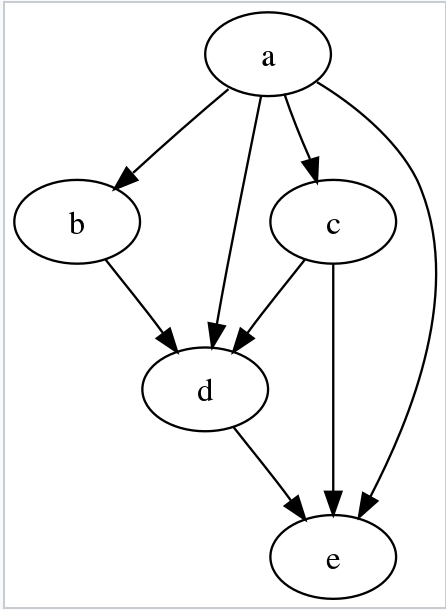
All these steps are captured in DAG ( Directed Acrylic graph ).
Let’s examine the definition of DAG.
In mathematics, particularly graph theory, and computer science, a directed acyclic graph (DAG) is a directed graph with no directed cycles. That is, it consists of vertices and edges (also called arcs), with each edge directed from one vertex to another, such that following those directions will never form a closed loop. A directed graph is a DAG if and only if it can be topologically ordered, by arranging the vertices as a linear ordering that is consistent with all edge directions. DAGs have numerous scientific and computational applications, ranging from biology (evolution, family trees, epidemiology) to information science (citation networks) to computation (scheduling).
Directed acyclic graphs are sometimes instead called acyclic-directed graphs or acyclic digraphs.

Image Source — Wikipedia
Source Wikipedia — https://en.wikipedia.org/wiki/Directed_acyclic_graph
The main takeaway about DAG is it’s not cyclic which means you can’t refer back to the same vertices. In Spark architecture of distributed setup, this is helpful because if any step is corrupted because of network or hardware failure that step can be recreated from the parent vertices and not complete flow needs to be recreated, as Spark maintains the lineage execution plan consists of stages and tasks, and it outlines the sequence of transformations and actions required to compute the final result. Spark employs various optimization techniques like pipelining and caching to minimize unnecessary re-computation and enhance performance. Because it's acyclic you can always recreate any failed or corrupt RDD from the transformation lineage information stored in Sprak.
Now that we have understood DAG let’s get back to our main topic of laziness and what it means in the context of spark.
The transformation we discussed earlier is of two types in Spark:
Narrow transformations
Wide transformations
Before understanding what is the narrow and wide transformation we will have to understand another term partition, for parallelism at the executor level spark breaks data into small datasets called partitions. A partition is a collection of data rows that sit on one physical machine in the distributed cluster. The data frame partition represents how data is physically distributed across clusters.
In most cases you don’t manipulate these partitions in DataFrame, you define your high-level transformations, and Spark decides how these will execute on the cluster. Having said that with the requirements of reducing the compute power and hence optimizing the cost on cloud setup, you will have to be cognizant and know the knobs which will efficiently run your job. We will discuss this topic again in the performance optimization section.
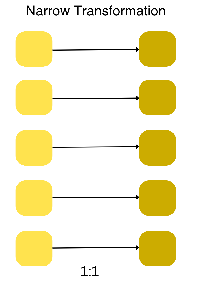
Narrow transformation
Each input partition will contribute to only one output partition.
1: 1 relationship. Each input partition contributes to only one output partition.
Examples of narrow transformation are select operation because it involves selecting specific columns from the DataFrame. Each partition processes its data independently, and there’s no need for data shuffling.
Remember that most transformation operations like filter, select, drop, and operations that don’t require interactions across partitions are considered narrow transformations in DataFrames as well. These operations can be performed efficiently without extensive data movement between partitions or machines in a distributed system over a network.

Narrow transformation
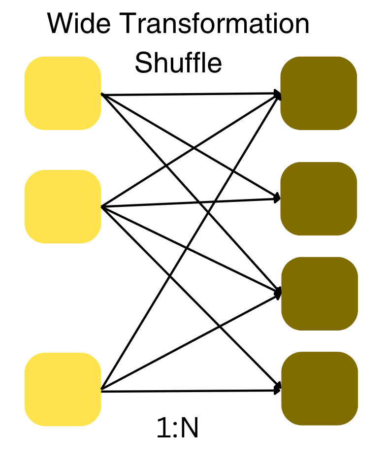
Wide transformation
Each input partition contributes to many output partitions 1: N.
Examples of wide transformation are groupBy and agg operations because they involve grouping the data by the column, which requires data to be shuffled and exchanged between partitions for aggregation.
Other examples of wide transformations in DataFrames include operations like join, orderBy (sorting operation), and anything that requires interactions between partitions and data redistribution.

Wide transform
Spark will exchange partition across clusters, hence shuffling. Shuffling causes the data to be exchanged over the network and hence a costly operation, while optimization is one of the first steps to identify how many shuffles occur in your job, whether they are necessary and how to avoid or minimize them.
Now in Spark, transformations and actions are two fundamental concepts that define the way data processing and computation are performed. Actions are operations that trigger the execution of transformations and produce results or effects. When an action is invoked on an RDD, Spark evaluates the entire lineage graph of transformations leading up to that RDD and starts the actual computation. Actions are eager operations, which means they lead to the execution of all pending transformations. Examples of actions include count, collect, saveAsTextFile, reduce, for each, and more. Actions return values or write data to external storage systems.
There are three kinds of actions:
Console display like count() , take(n) (n is the number of rows)
Collect data to native objects in respective language actions like collect() or toLocalIterator() is brought back to the driver program as a native data structure (like an array in most languages) in the respective language. This operation should be used with caution, especially when dealing with large datasets, as it moves all the data to the driver’s memory and can potentially cause memory issues.
Write-to-output data source actions like write or save are used to write the data in a DataFrame to an external data source, such as a file system, a database, or other supported storage formats.
Actions are typically used to trigger the execution of the logical plan that was built using transformations. These transformations define the sequence of operations to be applied to the data, and actions are what initiate the computation and return results.
Spark follows a lazy evaluation strategy, where transformations are not immediately executed. Instead, they are recorded as logical operations forming a DAG. Only when an action is encountered. Spark initiates the execution of transformations. The Catalyst Optimizer plays a key role in optimizing the execution process. It first optimizes the logical plan generated from the recorded transformations and then produces an optimized physical execution plan. This plan takes into account factors like predicate pushdown, data locality, and join optimizations.
While transformations define how data is modified or manipulated, actions trigger the execution of these transformations and yield results. This separation allows Spark to optimize the execution by fusing and rearranging transformations into an efficient physical execution plan, enhancing performance and resource utilization.

Image source — Databricks
Source — https://www.databricks.com/glossary/catalyst-optimizer
Spark has a catalyst optimizer which is similar to a query optimizer in a traditional relational database. The Catalyst Optimizer is a core component of the Apache Spark framework. It’s an advanced query optimization framework that optimizes the execution of relational queries in Spark SQL. Its primary goal is to transform the logical representation of a query into an optimized physical execution plan, thereby improving the performance of query processing.
Here’s how the Catalyst Optimizer works:
Query Parsing: Catalyst starts by parsing the SQL query or DataFrame/Dataset operations to build a logical plan that represents the high-level operations required to fulfill the query.
Logical Optimization: The logical plan undergoes a series of logical optimizations. These optimizations involve rewriting and simplifying the plan to remove unnecessary or redundant operations. Various rules and transformations are applied by Catalyst to achieve this.
Predicate Pushdown: Catalyst also performs predicate pushdown, which involves pushing filter conditions as close to the data source as possible, predicate pushdown reduces the considerable amount of data that needs to be processed.
Column Pruning: Catalyst identifies which columns are required to satisfy the query and eliminates unnecessary columns from the execution plan which minimizes data movement and improves query performance.
Physical Planning: After logical optimization, Catalyst generates multiple potential physical execution plans. These plans consider the available data sources, available computing resources, and possible join strategies. The best physical plan is then chosen out of these based on cost.
Cost-Based Optimization: Catalyst uses a cost-based optimization approach to estimate the cost of each physical plan. It takes into account factors like data distribution, data sizes, and available resources. The physical plan with the lowest estimated cost is selected.
Code Generation: Catalyst generates code for the selected physical plan. This code is usually in the form of Java bytecode or JVM-based code that gets executed on the Spark worker nodes.
Execution: The generated code is executed on the distributed Spark cluster to process the data and produce the query result.
By applying these optimization techniques, the Catalyst Optimizer significantly improves the performance of Spark SQL queries. It allows Spark to automatically choose the most efficient execution plan for a given query, taking into account the data and resources available in the cluster.
Let’s observe this lazy behavior of Spark with an example:
"""
 Data transformation
 Source of file: https://data.gov/
 @author Aruna Das
"""
from pyspark.sql import SparkSession
from pyspark.sql.functions import expr , col
import os
import logging

current_dir = os.path.dirname(__file__)
relative_path = "../data/SupplyChainGHGEmissionFactors_v1.2_NAICS_CO2e_USD2021.csv"
absolute_file_path = os.path.join(current_dir, relative_path)

# Step 1 - Creates a session on a local master
spark = SparkSession.builder.appName("Catalyst behaviour") \
    .master("local[*]").getOrCreate()

# set the log level to ERROR it will remove the clutter from the console
spark.sparkContext.setLogLevel("ERROR")

# Step 2 - Reads a CSV file with header, stores it in a dataframe
df = spark.read.csv(header=True, inferSchema=True,path=absolute_file_path)

# Step 3 - Cleanup. preparation
df = df.withColumnRenamed("Supply Chain Emission Factors without Margins", "efwom") \
       .withColumnRenamed("Margins of Supply Chain Emission Factors", "mef")\
       .withColumnRenamed("Supply Chain Emission Factors with Margins", "efwm")

# Step 4 - Transformation
df = df.withColumn("dmef", col("mef")) \
            .withColumn("mef2", expr("dmef * 2")) \
            .withColumn("efwm2", expr("efwom + mef2"))


df.show(5)

# Step 5 - Action
df.count()

df.explain()

spark.stop()
Flow chart representations of above code.

flow chart with transform
Results:- If you observe the project section, it shows the calculations required for additional fields in the code.

Results of the above transformation code
"""
 Data transformation with drop command
 Source of file: https://data.gov/
 @author Aruna Das
"""
from pyspark.sql import SparkSession
from pyspark.sql.functions import expr , col
import os
import logging

current_dir = os.path.dirname(__file__)
relative_path = "../data/SupplyChainGHGEmissionFactors_v1.2_NAICS_CO2e_USD2021.csv"
absolute_file_path = os.path.join(current_dir, relative_path)

# Step 1 - Creates a session on a local master
spark = SparkSession.builder.appName("Catalyst behaviour") \
    .master("local[*]").getOrCreate()

# set the log level to ERROR it will remove the clutter from the console
spark.sparkContext.setLogLevel("ERROR")

# Step 2 - Reads a CSV file with header, stores it in a dataframe
df = spark.read.csv(header=True, inferSchema=True,path=absolute_file_path)

# Step 3 - Cleanup. preparation
df = df.withColumnRenamed("Supply Chain Emission Factors without Margins", "efwom") \
       .withColumnRenamed("Margins of Supply Chain Emission Factors", "mef")\
       .withColumnRenamed("Supply Chain Emission Factors with Margins", "efwm")

# Step 4 - Transformation
df = df.withColumn("dmef", col("mef")) \
            .withColumn("mef2", expr("dmef * 2")) \
            .withColumn("efwm2", expr("efwom + mef2"))

df = df.drop("dmef","mef2","efwm2")

df.show(5)

# Step 5 - Action
df.count()

df.explain()

spark.stop()
Flow chart representation of the above code. The difference is in this code there is a drop statement for all the new columns calculated.

Flow chart of Transform with drop
Catalysts get a chance to analyze the complete operation because Spark doesn’t act until it sees an action. While creating the plan for executing Spark optimizer realizes that new columns which are computed are eventually dropped and not used in final results. Hence it decide to not even compute those.
I know it’s an extreme example (we are not computing a bunch of fields and then throwing away in production but you get the idea) you can infer other operations like filter predicate pushdown before join if optimizer spots downstream filter after joining two huge datasets . All of this is possible because of lazy nature of Spark it doesn’t start immediate execution of code as soon as it receives first instruction. It waits until action which gives Spark to analyze the complete ‘ask’ account for factors like data distribution, data sizes, and available resources and choose the best cost optimize path for physical execution at each executor machine.
Catalyst optimizer simplifies the flow diagram by eliminating the transformation section completely.

Flow chart adjusted after catalyst optimization
Results:- If you observe the explain plan, it reads the dataset and display on console without any computation or transformation phase, those operations are skipped because Spark’s Catalyst Optimizer may notice that the new columns are created and dropped without any intermediate actions. It may then optimize away these operations, recognizing that they have no impact on the final result.

Results of transformation with drop command.
You can find all the code at the location GitHub
Bonus- You will find the file name transformationExplain_union.py at the above GitHub location, this was an experimental code I was running which takes a CSV file of count 1016, using this original dataset and looping over with union function I created a bigger dataset of 1,017,016. Run the code with and without drop columns after transformation and record the time taken for these processes. The results are 26060 ms without drop function and 25835 ms with drop columns after transformation (as you already know, these results depend on machine capacity and other applications running on my machine when I was running, if you choose to run these scripts on your machine you might get different results). Well in this case union is the most taxing operation but you see the effect of optimization.
1. Creating a session ************ 1855

Number of orginal records .................... 1016

2. Loading original dataset ************ 3380

3. Building larger dataset ************ 56575

4. Clean-up complete************************ 202

5. Transformations  ************ 580

+---------------+--------------------+--------+--------------------+-----+-----+-----+---------------------+-----+-----+------------------+

|2017 NAICS Code|    2017 NAICS Title|     GHG|                Unit|efwom|  mef| efwm|Reference USEEIO Code| dmef| mef2|             efwm2|

+---------------+--------------------+--------+--------------------+-----+-----+-----+---------------------+-----+-----+------------------+

|         111110|     Soybean Farming|All GHGs|kg CO2e/2021 USD,...|1.223|0.103|1.326|               1111A0|0.103|0.206|             1.429|

|         111120|Oilseed (except S...|All GHGs|kg CO2e/2021 USD,...|1.223|0.103|1.326|               1111A0|0.103|0.206|             1.429|

|         111130|Dry Pea and Bean ...|All GHGs|kg CO2e/2021 USD,...|2.874|0.134|3.007|               1111B0|0.134|0.268|3.1420000000000003|

|         111140|       Wheat Farming|All GHGs|kg CO2e/2021 USD,...|2.874|0.134|3.007|               1111B0|0.134|0.268|3.1420000000000003|

|         111150|        Corn Farming|All GHGs|kg CO2e/2021 USD,...|2.874|0.134|3.007|               1111B0|0.134|0.268|3.1420000000000003|

+---------------+--------------------+--------+--------------------+-----+-----+-----+---------------------+-----+-----+------------------+

only showing top 5 rows


Record count of larger dataset.................... 1017016

6. Action called  ************ 26060

== Physical Plan ==

Union

:- *(1) Project [2017 NAICS Code#16, 2017 NAICS Title#17, GHG#18, Unit#19, Supply Chain Emission Factors without Margins#20 AS efwom#16045, Margins of Supply Chain Emission Factors#21 AS mef#16054, Supply Chain Emission Factors with Margins#22 AS efwm#16063, Reference USEEIO Code#23, Margins of Supply Chain Emission Factors#21 AS dmef#16072, (Margins of Supply Chain Emission Factors#21 * 2.0) AS mef2#16082, (Supply Chain Emission Factors without Margins#20 + (Margins of Supply Chain Emission Factors#21 * 2.0)) AS efwm2#16093]

:  +- FileScan csv [2017 NAICS Code#16,2017 NAICS Title#17,GHG#18,Unit#19,Supply Chain Emission Factors without Margins#20,Margins of Supply Chain Emission Factors#21,Supply Chain Emission Factors with Margins#22,Reference USEEIO Code#23] Batched: false, DataFilters: [], Format: CSV, Location: InMemoryFileIndex(1 paths)[file:/home/aruna/spark/app/article/SparkSeries/data/SupplyChainGHGEm..., PartitionFilters: [], PushedFilters: [], ReadSchema: struct<2017 NAICS Code:int,2017 NAICS Title:string,GHG:string,Unit:string,Supply Chain Emission F...

:- *(2) Project [2017 NAICS Code#45, 2017 NAICS Title#46, GHG#47, Unit#48, Supply Chain Emission Factors without Margins#49 AS efwom#33174, Margins of Supply Chain Emission Factors#50 AS mef#34174, Supply Chain Emission Factors with Margins#51 AS efwm#34175, Reference USEEIO Code#52, Margins of Supply Chain Emissio

 ++++++++++++ with drop command +++++++++

1. Creating a session ************ 2146

Number of orginal records .................... 1016

2. Loading original dataset ************ 4352

3. Building larger dataset ************ 59908

4. Clean-up complete************************ 187

5. Transformations  ************ 555

+---------------+--------------------+--------+--------------------+-----+-----+-----+---------------------+

|2017 NAICS Code|    2017 NAICS Title|     GHG|                Unit|efwom|  mef| efwm|Reference USEEIO Code|

+---------------+--------------------+--------+--------------------+-----+-----+-----+---------------------+

|         111110|     Soybean Farming|All GHGs|kg CO2e/2021 USD,...|1.223|0.103|1.326|               1111A0|

|         111120|Oilseed (except S...|All GHGs|kg CO2e/2021 USD,...|1.223|0.103|1.326|               1111A0|

|         111130|Dry Pea and Bean ...|All GHGs|kg CO2e/2021 USD,...|2.874|0.134|3.007|               1111B0|

|         111140|       Wheat Farming|All GHGs|kg CO2e/2021 USD,...|2.874|0.134|3.007|               1111B0|

|         111150|        Corn Farming|All GHGs|kg CO2e/2021 USD,...|2.874|0.134|3.007|               1111B0|

+---------------+--------------------+--------+--------------------+-----+-----+-----+---------------------+

only showing top 5 rows


Record count of larger dataset.................... 1017016

6. Action called  ************ 25835

== Physical Plan ==

Union

:- *(1) Project [2017 NAICS Code#16, 2017 NAICS Title#17, GHG#18, Unit#19, Supply Chain Emission Factors without Margins#20 AS efwom#16045, Margins of Supply Chain Emission Factors#21 AS mef#16054, Supply Chain Emission Factors with Margins#22 AS efwm#16063, Reference USEEIO Code#23]

:  +- FileScan csv [2017 NAICS Code#16,2017 NAICS Title#17,GHG#18,Unit#19,Supply Chain Emission Factors without Margins#20,Margins of Supply Chain Emission Factors#21,Supply Chain Emission Factors with Margins#22,Reference USEEIO Code#23] Batched: false, DataFilters: [], Format: CSV, Location: InMemoryFileIndex(1 paths)[file:/home/aruna/spark/app/article/SparkSeries/data/SupplyChainGHGEm..., PartitionFilters: [], PushedFilters: [], ReadSchema: struct<2017 NAICS Code:int,2017 NAICS Title:string,GHG:string,Unit:string,Supply Chain Emission F...

:- *(2) Project [2017 NAICS Code#45, 2017 NAICS Title#46, GHG#47, Unit#48, Supply Chain Emission Factors without Margins#49 AS efwom#30167, Margins of Supply
Again knowing the internal behaviors of Spark like it has transformations and actions. Two types of transformations narrow and wide , one is more costlier (wide) in terms of network shuffle than other what are those functions which are narrow vs wide? How catalyst optimizer works? Spark is fundamentally lazy doesn’t act until sees an action command in the pipeline. These inner workings of knowhows will help you write more efficient and optimized pipelines whether batch or streaming, as the same principles apply to both contexts.
If establishing a connection interests you, you can find my LinkedIn profile at the following link: https://www.linkedin.com/in/arunadas29/
